Icosahedral grid-based density estimation Spatial density estimation algorithm based on rotation of icosahedral grids.

Any points set can be binned to an icosahedral grid (i.e. number of incidences can be counted), which will be dependent on the exact positions of grid cells. Rotating the grid in 3d space will result in a different distribution of counts. This distribution can be resampled to a standard orientation structure. The size of the icosahedral grid cells act as a bandwidth parameter.

Discretization with iteratively rotated icosahedral grids

Usage

gridensity(x, y, out, trials = 100, FUN = mean)

grapply(x, out, ...)

# S4 method for class 'data.frame,SpatRaster'
grapply(
  x,
  out,
  y,
  coords = c("long", "lat"),
  iter = 100,
  FUN = function(x) table(x$cell),
  APP = mean,
  miss = NA,
  APP.args = NULL,
  counter = TRUE,
  FUN.args = NULL
)

# S4 method for class 'data.frame,trigrid'
grapply(
  x,
  out,
  y = out,
  coords = c("long", "lat"),
  iter = 100,
  FUN = function(x) table(x$cell),
  APP = mean,
  miss = NA,
  APP.args = NULL,
  counter = TRUE,
  FUN.args = NULL
)

# S4 method for class 'matrix,SpatRaster'
grapply(x, out, ...)

# S4 method for class 'matrix,trigrid'
grapply(x, out, ...)

# S4 method for class 'data.frame,missing'
grapply(x, out, y, ...)

# S4 method for class 'matrix,missing'
grapply(x, out, y, ...)

Arguments

x

Matrix of longitude, latitude data, sf class, or SpatialPoints Point cloud.

y

trigrid or hexagrid An icosahedral grid.

out

trigrid, hexagrid or SpatRasteroutput structure. If not given, then the input argument

trials

numeric value, the number of iterations.

FUN

function The function to be applied on the iteration results. It defaults to the number of points, but it can be used to

...

Arguments passed to class-specific methods.

coords

character Column names to find longitude and latiude variables in x.

iter

numeric Value, the number of iterations.

APP

function The function to be applied on the iteration results. If set to NULL, it will return the stack of results for subsequent processing.

miss

numeric A single default value used in positions in out where no value is produced by FUN in an iteration trial.

APP.args

list Additional arguments passed to APP.

counter

logical Should a loop counter be shown?

FUN.args

list Additional arguments passed to FUN.

Value

Either named numeric vector, or a SpatRaster object. If FUN is set to NULL, the output will be either a matrix or SpatRaster.

Details

The implemented algorithm 1) takes a point cloud (x)) and an icosahedral grid y 2) randomly rotates the icosahedral grid, 3) looks up the points falling on grid cells, 4) resamples the grid to a constant orientation object (either trigrid, hexagrid or SpatRaster). Steps 2-4 are repeated trial times, and then FUN is applied to every vector of values that have same spatial position.

Simple discretization of spatial data is subject to error due to the random assignment to grid cells. grapply offers a framework for the Monte Carlo estimation of the expectation of a function that normally can be applied to a discretized set of points. This function FUN takes the input the data.frame (or matrix, which will be coerced into one) as argument, with the addition of a new variable cells, which includes face identifiers for the point set given the random grid rotation (the output of locate). See examples for a step-by-step description.

Examples

# example to be run if terra is present
if(requireNamespace("terra", quietly=TRUE)){

 # randomly generated points
 x <- rpsphere(100, output="polar")

 # bandwidth grid
 gr <- hexagrid(deg=13)

 # output structure
 out <- terra::rast(res=5)

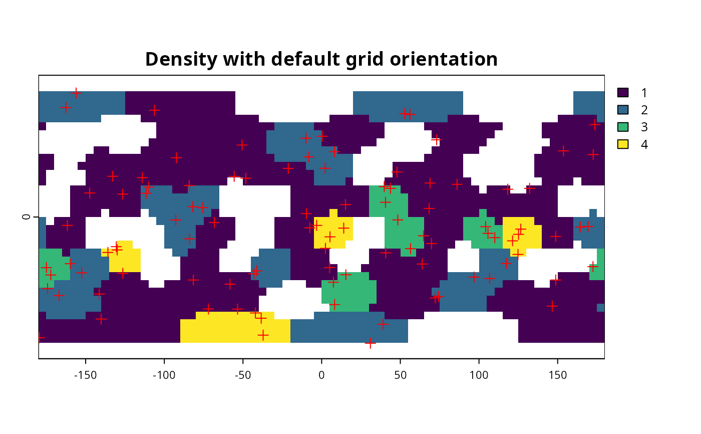
 # Manual example - for understanding what FUN is doing
 cell<- locate(gr, x)
yNew <- cbind(as.data.frame(x), cell=cell)
 # this is the default function (here named CellCount)
 CellCount <- function(x) table(x$cell)
 counts <- CellCount(yNew)
 # create facelayer
 fl <- facelayer(gr, counts)

 # and resample
 oneOut <- icosa::resample(fl, out)
 terra::plot(oneOut, main="Density with default grid orientation")
 points(x, pch=3, col="red")

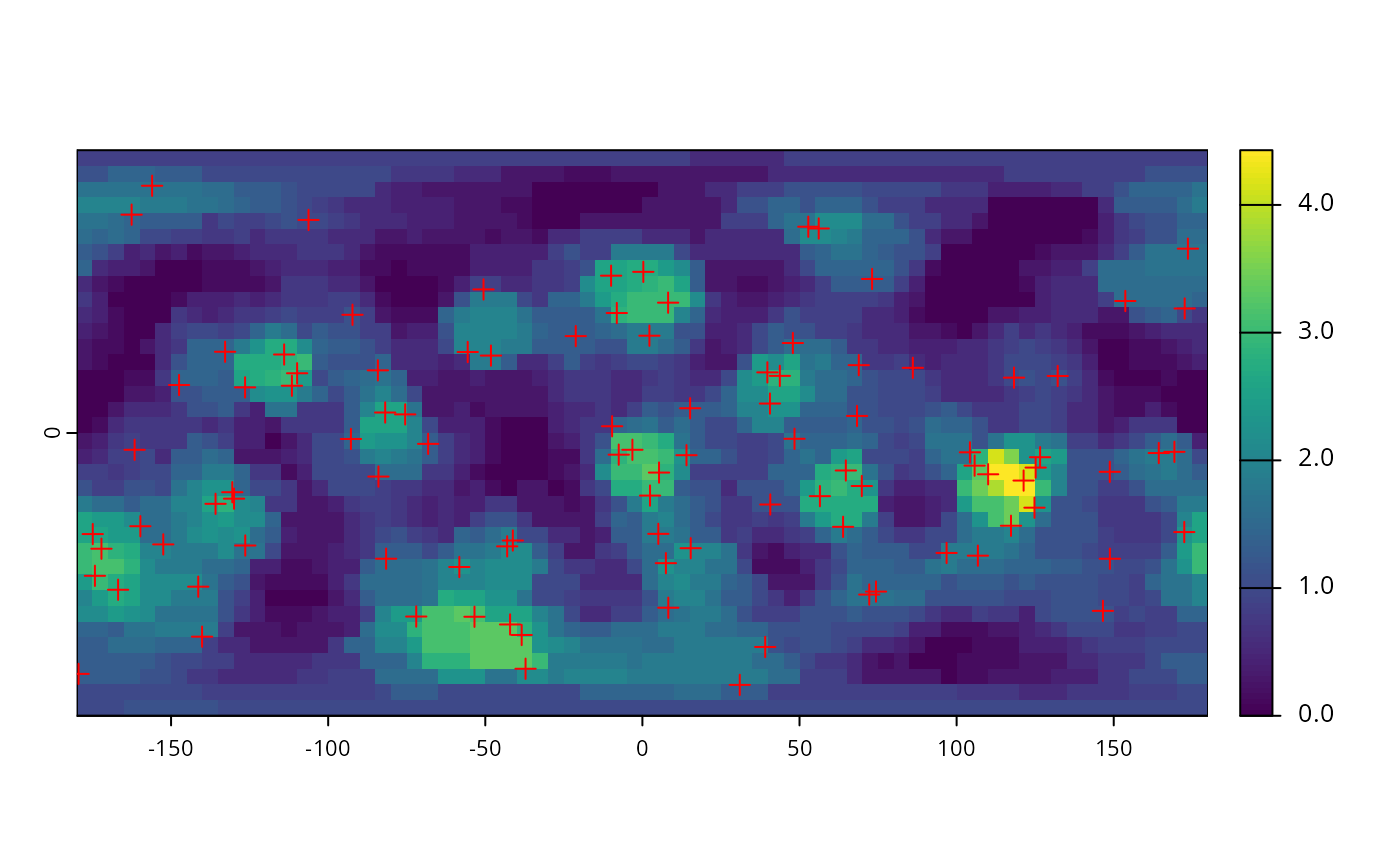
 # for density estimation
 o <- grapply(x=x, out=out,y=gr,  iter=7, FUN=CellCount, miss=0)

 # visualize results
 terra::plot(o)
 points(x, pch=3, col="red")
}
#> Selecting hexagrid with tessellation vector: c(3).
#> Mean edge length: 13.35 degrees.

#> 1 
2 
3 
4 
5 
6 
7